Speech Processing using MATLAB, Part 1

Contents

Short-Time Speech Measurements, Windows

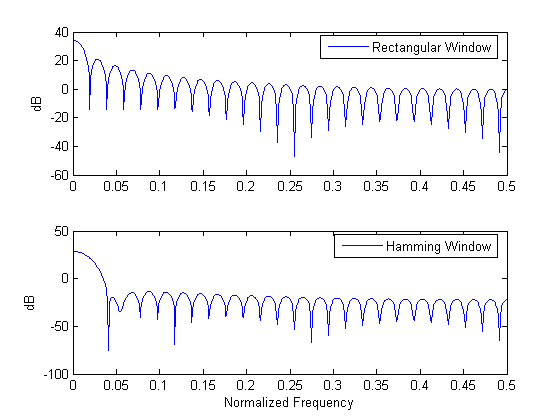
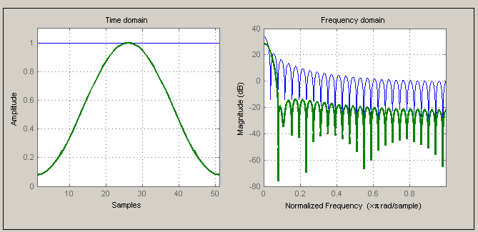
The choice of the window in short-time speech processing determines the nature of the measurement representation. A long window would result in very little changes of the measurement in time whereas the measurement with a short window would not be sufficiently smooth. Two representative windows are demonstrated, Rectangular and Hamming. The latter has almost twice the bandwidth of the former, for the same length. Furthermore, the attenuation for the Hamming window outside the passband is much greater.

% General Settings, path settings, data loading
speechDemo_workspace_config;
phons = readdata(wavpath, '_', 6, 'phonemes');

% Sampling frequency in Hz (for the data used in this demo i.e TIMIT database signals)
Fs = 16000;

% Rectangular and Hamming window, chosen from the variety of windows
% offered in MATLAB.
wRect = rectwin(51);
wHamm = hamming(51);

% Calculate the magnitude of the Fast Fourier Transform of the windows
fftLength = 1024;
magFWHamm = abs(fft(wHamm, fftLength));
magFWRect = abs(fft(wRect, fftLength));

subplot(2,1,1);
plot(linspace(0,0.5,ceil(fftLength/2)), 20*log10(magFWRect(1:ceil(fftLength/2))));
ylabel('dB');
legend('Rectangular Window');
subplot(2,1,2);
plot(linspace(0,0.5,ceil(fftLength/2)), 20*log10(magFWHamm(1:ceil(fftLength/2))));
ylabel('dB');
xlabel('Normalized Frequency');
legend('Hamming Window');

% Window visualization tool by MATLAB
wvtool(wRect, wHamm);

rootpath =

C:\Nassos\Didaktoriko\Courses_Didaktoriko\PatternRecognition_Didaktoriko\work\speech_demo\speech_course_2004

Short-Time Speech Measurements, Short-Time energy calculation

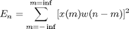
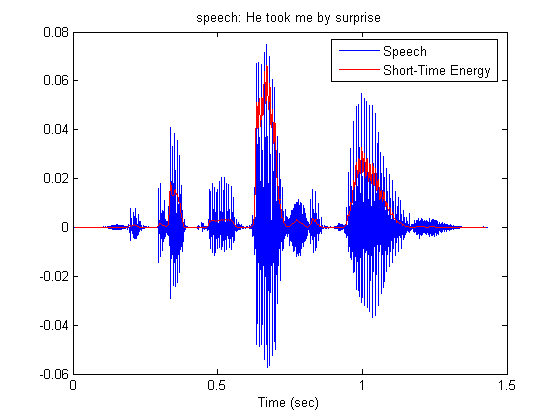
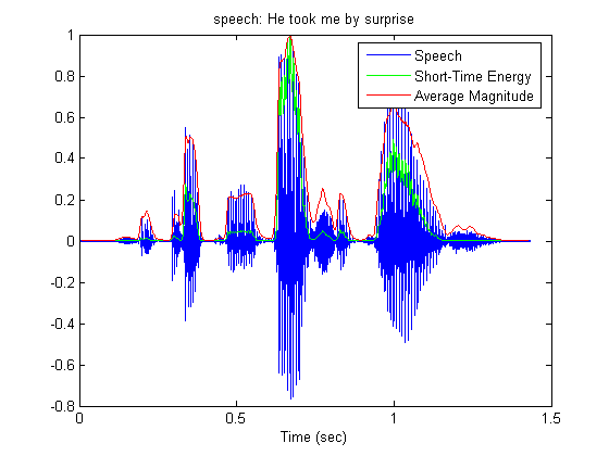
Short-Time energy is a simple short-time speech measurement. It is defined as:

This measurement can in a way distinguish between voiced and unvoiced speech segments, since unvoiced speech has significantly smaller short- time energy. For the length of the window a practical choice is 10-20 msec that is 160-320 samples for sampling frequency 16kHz. This way the window will include a suitable number of pitch periods so that the result will be neither too smooth, nor too detailed.

% A sentence stored in SPHERE format is read. The sentence is :
% 'He took me by surprise'. A function of voicebox is used.
speechSignal = readsph(fullfile(wavpath,'SI1899a.WAV'));

% A hamming window is chosen
winLen = 301;
winOverlap = 300;
wHamm = hamming(winLen);

% Framing and windowing the signal without for loops.
sigFramed = buffer(speechSignal, winLen, winOverlap, 'nodelay');
sigWindowed = diag(sparse(wHamm)) * sigFramed;

% Short-Time Energy calculation
energyST = sum(sigWindowed.^2,1);

% Time in seconds, for the graphs
t = [0:length(speechSignal)-1]/Fs;

subplot(1,1,1);
plot(t, speechSignal);
title('speech: He took me by surprise');
xlims = get(gca,'Xlim');

hold on;

% Short-Time energy is delayed due to lowpass filtering. This delay is
% compensated for the graph.
delay = (winLen - 1)/2;
plot(t(delay+1:end - delay), energyST, 'r');
xlim(xlims);
xlabel('Time (sec)');
legend({'Speech','Short-Time Energy'});
hold off;

Short-Time Speech Measurements, Short-Time energy calculation, window length, Hamming

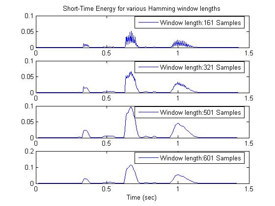
Effects of the choice of window length are demonstrated. As the length increases, short-time energy becomes smoother, as expected. It should be noticed that the measurement is not taken for every sample. Due to the lowpass character of the window, short-time energy is actually bandlimited to the bandwidth of the window, which is much smaller than 16 KHz. Actually for the lengths we are interested in, it is less than 160 Hz. So, we could calculate the energy every 50 samples, that is with 320 Hz frequency for 16kHz speech sampling frequency.

% Energy is calculated every period samples.
period = 50;

% 4 different window lengths
winLens = [161 321 501 601];
nWindows = length(winLens);

k = 0;
for iWinLen = winLens
    k = k+1;
    wHamm = hamming(iWinLen);

    % Short-Time energy calculation
    ienergyST = STenergy(speechSignal, wHamm, iWinLen - period);

    % Display results
    subplot(nWindows, 1, k);

    delay = (iWinLen - 1)/2;
    plot(t(delay+1:period:end - delay), ienergyST);
    if (k==1)
        title('Short-Time Energy for various Hamming window lengths')
    end
    if (k==4)
        xlabel('Time (sec)')
    end

    legend(['Window length:',num2str(iWinLen),' Samples'])
end

Short-Time Speech Measurements, Short-Time energy calculation, window length, Rectangular

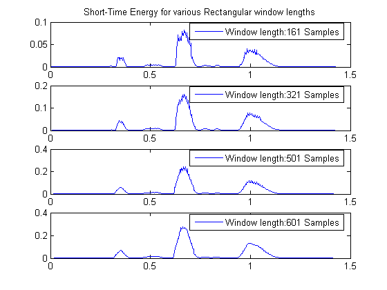
The rectangular window has smaller bandwidth for the same length, compared to the Hamming window. So the results are expected to be smoother. In any case, as the length of the window increases short-time energy is less detailed.

% Energy is calculated every period samples.
period = 50;

% 4 different window lengths
winLens = [161 321 501 601];
nWindows = length(winLens);

k = 0;
for iWinLen = winLens
    k = k+1;
    wRect = rectwin(iWinLen);

    % Short-Time energy calculation
    ienergyST = STenergy(speechSignal, wRect, iWinLen-period);

    % Display results
    subplot(nWindows, 1, k);
    delay = (iWinLen - 1)/2;
    plot(t(delay+1:period:end - delay), ienergyST);
    if (k==1)
        title('Short-Time Energy for various Rectangular window lengths')
    end
    legend(['Window length:',num2str(iWinLen),' Samples']);
end

Short-Time Speech Measurements, Average Magnitude calculation

Average magnitude function defined as

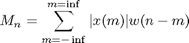
does not emphasize large signal levels so much as short-time energy since its calculation does not include squaring. The signals in the graphs are normalized.

winLen = 301;
winOverlap = 300;
wHamm = hamming(winLen);
magnitudeAv = STAmagnitude(speechSignal, wHamm, winOverlap);

subplot(1,1,1);
plot(t, speechSignal/max(abs(speechSignal)));
title('speech: He took me by surprise');
hold on;
delay = (winLen - 1)/2;
plot(t(delay+1:end-delay), energyST/max(energyST), 'g');
plot(t(delay+1:end-delay), magnitudeAv/max(magnitudeAv), 'r');
legend('Speech','Short-Time Energy','Average Magnitude');
xlabel('Time (sec)');
hold off;

Short-Time Speech Measurements, Average Zero-Crossing Rate

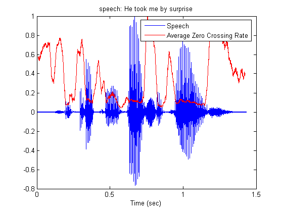
Average Zero-Crossing Rate is defined as

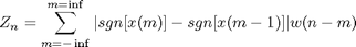
w(n) = 1/2N, 0 <= n <= N-1 This measure could allow the discrimination between voiced and unvoiced regions of speech, or between speech and silence. Unvoiced speech has in general, higher zero-crossing rate. The signals in the graphs are normalized.

wRect = rectwin(winLen);
ZCR = STAzerocross(speechSignal, wRect, winOverlap);

subplot(1,1,1);
plot(t, speechSignal/max(abs(speechSignal)));
title('speech: He took me by surprise');

hold on;
delay = (winLen - 1)/2;

plot(t(delay+1:end-delay), ZCR/max(ZCR),'r');
xlabel('Time (sec)');
legend('Speech','Average Zero Crossing Rate');
hold off;

Short-Time Speech Measurements, Short-Time Autocorrelation, Varying Window Length

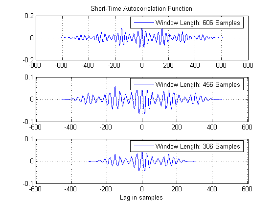
Short-time autocorrelation is defined as

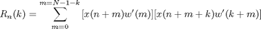
and is actually the autocorrelation of a windowed speech segment. The window used is the rectangular. Notice the attenuation of the autocorrelation as the window length becomes shorter. This is expected, since the number of the samples used in the calculation decreases.

% Three speech segments, of different length.
ss1 = speechSignal(16095:16700);
ss2 = speechSignal(16095:16550);
ss3 = speechSignal(16095:16400);

% Calculation of the short time autocorrelation
[ac1, lags1] = xcorr(ss1);
[ac2, lags2] = xcorr(ss2);
[ac3, lags3] = xcorr(ss3);

subplot(3,1,1);
plot(lags1, ac1);
legend('Window Length: 606 Samples')
title('Short-Time Autocorrelation Function')
grid on;
subplot(3,1,2);
plot(lags2, ac2);
xlim([lags1(1) lags1(end)]);
legend('Window Length: 456 Samples')
grid on;
subplot(3,1,3);
plot(lags3, ac3);
xlim([lags1(1) lags1(end)]);
legend('Window Length: 306 Samples')
xlabel('Lag in samples')
grid on;

Short-Time Speech Measurements, Short-Time Autocorrelation, Voiced and Unvoiced Speech

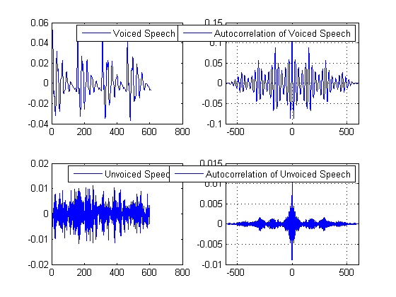
The property of the short-time autocorrelation to reveal periodicity in a signal is demonstrated. Notice how the autocorrelation of the voiced speech segment retains the periodicity. On the other hand, the autocorrelation of the unvoiced speech segment looks more like noise. In general, autocorrelation is considered as a robust indicator of periodicity.

% An unvoiced speech segment.
ss4 = speechSignal(12200:12800);
[ac4, lags4] = xcorr(ss4);

subplot(2,2,1);
plot(ss1);
legend('Voiced Speech')
subplot(2,2,2);
plot(lags1, ac1);
xlim([lags1(1) lags1(end)]);
legend('Autocorrelation of Voiced Speech')
grid on;
subplot(2,2,3);
plot(ss4);
legend('Unvoiced Speech')
subplot(2,2,4);
plot(lags4, ac4);
xlim([lags1(1) lags1(end)]);
legend('Autocorrelation of Unvoiced Speech')
grid on;

Spectrogram, FFT of speech

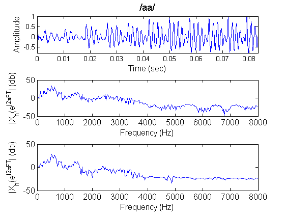
Representation of speech in the frequency domain is demonstrated. The importance FFT as a computational tool becomes also clear.

speechDemo_config_spec_params;

% Isolated phonemes wav files list , as a cell by get_WavList() function
wavname=get_WavList(wavpath);

subplot(1,1,1);

% Next is shown a sample way to loop over selected phonemes and do some kind of processing after reading
% create a list of selected phonemes to process
selected_phonindx=[1:length(wavname)]; 	% in this list put all the phons
for index=1:length(selected_phonindx) 	% loop over the selected phons

	wfile=[wavpath,filesep,wavname{index}]; 		% construct full wav file name
	label=getfield_byfname(wavname,index,recsep,labelinds); % use a mapping function to get the label out of the filename

	% raw read data, can use also readsph()
	fid=fopen(wfile,'r');
	y=fread(fid,inf,'short');% no header in these phoneme wavs  (NOTE: this isnt the case for the wav phrases)
	y=y(:);  		 % make sure its a column
	y=y/max(y);		 % normalize
	fclose(fid);

	% take the initiative to process data ...!
	% by placing in here your own functions/code
	% e.g. you can select some code from the current script and loop around different phonemes to
	% to observe their characteristics (spectrogram, lpc, etc)

end

% Select a specific phoneme by its index
index=2;
% Construct its filename
wfile=[wavpath,filesep,wavname{index}];
% find label from filename
label=getfield_byfname(wavname,index,recsep,labelinds);

% raw read data
fid=fopen(wfile,'r');
y=fread(fid,inf,'short'); % no header in these phoneme wavs
y=y(:);  y=y/max(y);
fclose(fid);
titlestr=['/',label,'/'];

% Fft the whole phoneme
FSignal=fft(y,2^9);
% In case you want the phase too, do not forget to unwrap it !
% Phase=unwrap(angle(FSignal));
FSignal=FSignal(1:ceil(length(FSignal)/2));

% Window the signal with hamming and apply Fast Fourier Transform
HFSignal=fft(y.*hamming(length(y)),2^9);

subplot(3,1,1),
plot_speech(y,Fs,linewidth,titlestr,fontsize);
subplot(3,1,2),
plot_spectrum(FSignal,Fs,linewidth,'',fontsize,'b');
subplot(3,1,3),
plot_spectrum(HFSignal(1:ceil(length(HFSignal)/2)),Fs,linewidth,'',fontsize,'b');

Spectrogram, FFT of speech, Long window

Demonstration of the calculation of the spectrum using long windows, either Hamming or rectangular

% FFT in relatively long window, rectangular window
winlen=512; %  32msec in 16KHz
% Do parallel processing by buffering
FrameSignal = buffer(y,winlen,round(winlen/3));
FFrameSignal = fft(FrameSignal,1024);
% No need to keep the whole spectrum
FFrameSignal = FFrameSignal(1:ceil(size(FSignal,1)/2),:);

% fft in relatively long window ,  hamming window
winlen = 512; %  32msec in 16KHz
win = hamming(winlen);
HFrameSignal = buffer(y,winlen,round(winlen/3));
% Windowing the signal without loops
HWinFrameSignal = diag(sparse(win))*HFrameSignal; % tony's trick for windowing the signal
HFFrameSignal = fft(HWinFrameSignal,1024);
HFFrameSignal = HFFrameSignal(1:ceil(size(HFFrameSignal,1)/2),:);

% plot all frames sequentially , both time and abs spectra,  both rectangular and Hamming windowd signals
plot_frames_SigFreq_HF(FFrameSignal,HFFrameSignal,FrameSignal,HWinFrameSignal,Fs,linewidth,fontsize,1,2)

Spectrogram, FFT of speech, Short window

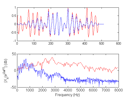
Demonstration of the calculation of the spectrum using short windows, either Hamming or rectangular.

% rectangular window
FFrameSignal=[];
FrameSignal=[];
winlen=32; % 4msec in 16KHz
FrameSignal=buffer(y,winlen,round(winlen/3));
FFrameSignal = fft(FrameSignal,1024);
FFrameSignal=FFrameSignal(1:ceil(size(FFrameSignal,1)/2),:);

% FFT in relatively short window
% hamming window
winlen=32; % 4msec in 16KHz
win=hamming(winlen);
HFrameSignal=buffer(y,winlen,round(winlen/3));
HWinFrameSignal = diag(sparse(win))*HFrameSignal; % tony's trick for windowing the signal
HFFrameSignal = fft(HWinFrameSignal,1024);

plot_frames_SigFreq_HF(FFrameSignal,HFFrameSignal,FrameSignal,HWinFrameSignal,Fs,linewidth,fontsize,1,0.30)

Spectrogram, A longer phrase

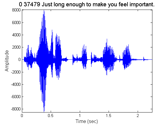
Frequency domain representation of a longer speech phrase. Firstly, the phrase is plotted.

% Read transcription from corresponding txt file and store it
fid= fopen([fullfile(phrase_datapath,phrase),'.txt'],'rt');
transcription=fgetl(fid);
fclose(fid);

% Raw wav read  instead of wavread (NOTE: phrase wavs have header, in contrast with previous case i.e. phonemes)
fid=fopen([fullfile(phrase_datapath,phrase),'.wav'],'r');
fread(fid,skiplen,'int'); % who cares about the header
y=fread(fid,inf,'short'); % get the binary
fclose(fid);

% Plot the whole phrase
titlestr=transcription;
subplot(1,1,1), plot_speech(y,Fs,linewidth,titlestr,fontsize); hold on;

Spectrogram, A longer phrase, Add phonetic transcription

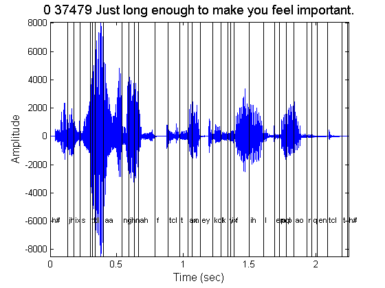
% Open *.phn file, that contains the phoneme labels with their boundaries
fid= fopen([fullfile(phrase_datapath,phrase),'.phn'],'rt');
while 1,
	% process each line
	line = fgetl(fid);
	if ~ischar(line), return; end
	% use wsep to split records
	wsepind = strfind(line,wsep);
	% place the labels in the appropriate positions using text
	ht = text(mean(str2num(line(1:wsepind(1)))/Fs),0.7*min(y),line(wsepind(2):end));
	% set the font large enough to be able to see them, but keep them alligned
	set(ht,'fontsize',fontsize_infigtext);
	% draw lines at bounds
	plot(str2num(line(1:wsepind(1)))/Fs*ones(1,10),linspace(min(y),max(y),10),'k')
end
fclose(fid);

Spectrogram, Narrowband or Wideband

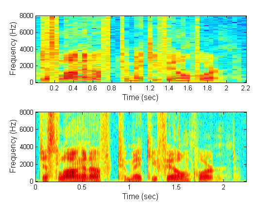
Demonstration of the spectrogram, narrowband or wideband. Notice that the latter has better time-resolution (since it uses a short window in time) but worse frequency resolution. In the case of the wideband spectrogram,the window is of about the same duration as the pitch period. Notice the vertical striations due to this fact. For unvoiced speech there are no vertical striations. Function specgram of MATLAB is used.

% Long window in time - Narrowband
t_window_narrowband = .05;		% window - time
t_overlap_narrowband = .001;
window_narrowband = t_window_narrowband*Fs;	% window samps
noverlap_narrowband = t_overlap_narrowband*Fs;
nfft_narrowband = 1024;

window = window_narrowband;
noverlap = noverlap_narrowband;
nfft = nfft_narrowband;

subplot(2,1,1);
specgram(y,nfft,Fs,window,noverlap);
xlabel('Time (sec)','fontsize',fontsize);
ylabel('Frequency (Hz)','fontsize',fontsize);

% Spectrogram, Wideband, short window in time
t_window_wideband = .005;		% window - time
t_overlap_wideband = .001;
window_wideband = t_window_wideband*Fs;	% window samps
noverlap_wideband = 1; %t_overlap_wideband*Fs;
nfft_wideband = 8192;

window = window_wideband;
noverlap = noverlap_wideband;
nfft = nfft_wideband;
subplot(2,1,2)
specgram(y,nfft,Fs,window,noverlap);
xlabel('Time (sec)','fontsize',fontsize);
ylabel('Frequency (Hz)','fontsize',fontsize);

Linear Prediction, Autocorrelation method

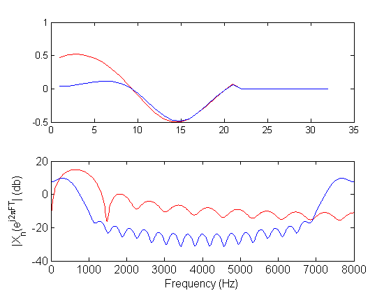
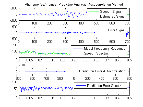
Linear predictive analysis of speech is demonstrated. The methods used are either the autocorrelation method or the covariance method. The autocorrelation method assumes that the signal is identically zero outside the analysis interval (0<=m<=N-1). Then it tries to minimize the prediction error wherever it is nonzero, that is in the interval 0<=m<=N-1+p, where p is the order of the model used. The error is likely to be large at the beginning and at the end of this interval. This is the reason why the speech segment analyzed is usually tapered by the application of a Hamming window, for example. For the choice of the window length it has been shown that it should be on the order of several pitch periods to ensure reliable results. One advantage of this method is that stability of the resulting model is ensured. The error autocorrelation and spectrum are calculated as a measure of the whiteness of the prediction error.

% Voiced sound
phons = readdata(wavpath, '_', 6, 'phonemes');
x = phons.aa{5}(200:890);
len_x = length(x);

% The signal is windowed
w = hamming(len_x);
wx = w.*x;

% Lpc autocorrelation method
order = 20;

% LPC function of MATLAB is used
[lpcoefs, errorPow] = lpc(wx, order);

% The estimated signal is calculated as the output of linearly filtering
% the speech signal with the coefficients estimated above
estx = filter([0 -lpcoefs(2:end)], 1, [wx; zeros(order,1)]);

% The prediction error is estimated in the interval 0<=m<=N-1+p
er = [wx; zeros(order,1)] - estx;

%Prediction error energy in the same interva
erEn = sum(er.^2);

% Autocorrelation of the prediction error
[acs,lags] = xcorr(er);

% Calculate the frequency response of the linear prediction model
[H, W] = freqz(sqrt(erEn), lpcoefs(1:end), 513);

% Calculate the spectrum of the windowed signal
S = abs(fft(wx,1024));

% Calculate the spectrum of the error signal
eS = abs(fft(er,1024));

% Display results
subplot(5,1,1);
plot([wx; zeros(order,1)],'g');
title('Phoneme /aa/ - Linear Predictive Analysis, Autocorrelation Method');
hold on;
plot(estx);
hold off;
xlim([0 length(er)])
legend('Speech Signal','Estimated Signal');
subplot(5,1,2);
plot(er);
xlim([0 length(er)])
legend('Error Signal');
subplot(5,1,3);
plot(linspace(0,0.5,513), 20*log10(abs(H)));
hold on;
plot(linspace(0,0.5,513), 20*log10(S(1:513)), 'g');
legend('Model Frequency Response','Speech Spectrum')
hold off;
subplot(5,1,4);
plot(lags, acs);
legend('Prediction Error Autocorrelation')
subplot(5,1,5);
plot(linspace(0,0.5,513), 20*log10(eS(1:513)));
legend('Prediction Error Spectrum')

Linear Prediction, Covariance method

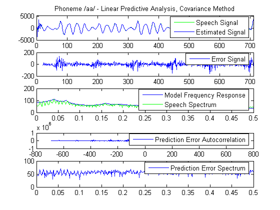
Demonstration of the covariance method for linear prediction. Compared to the autocorrelation method, the difference of the covariance method is that it fixes the interval over which the mean - square prediction error is minimized and speech is not taken to be zero outside this interval. Stability of the resulting model cannot be guaranteed but usually for sufficiently large analysis interval, the predictor coefficients will be stable. The error autocorrelation and spectrum are calculated as a measure of its whiteness.

x = phons.aa{5}(200-order:890);
Fs = 16000;
len_x = length(x);

% Function lpccovar of voicebox is used
[lpccovarcoefs, lpccovarer] = lpccovar(x, order);

% The estimated signal is calculated as the output of linearly filtering
% the speech signal with the coefficients estimated above
estx = filter([0 -lpccovarcoefs(2:end)], 1, x);

% Prediction error in the analysis frame
er = x(order+1:end) - estx(order+1:end);

% Prediction error energy estimated within the analysis frame (square of the
% Filter Gain)
erEn = sum(er.^2);
% Prediction error Autocorrelation
[acs,lags] = xcorr(er);

% Frequency response of the prediction model
[H, W] = freqz(sqrt(erEn), lpccovarcoefs(1:end), 513);
% Spectrum of windowed speech
S = abs(fft(wx,1024));
% Spectrum of prediction error
eS = abs(fft(er,1024));

subplot(5,1,1);
plot(x, 'g');
title('Phoneme /aa/ - Linear Predictive Analysis, Covariance Method');
hold on;
plot(estx)
xlim([0 length(x)])
legend('Speech Signal','Estimated Signal');
hold off
subplot(5,1,2);
plot(order+1:length(x), er);
xlim([0 length(x)])
legend('Error Signal');
subplot(5,1,3);
plot(linspace(0,0.5,513), 20*log10(abs(H)));
hold on;
plot(linspace(0,0.5,513), 20*log10(S(1:513)), 'g');
legend('Model Frequency Response','Speech Spectrum')
subplot(5,1,4);
plot(lags, acs);
legend('Prediction Error Autocorrelation')
subplot(5,1,5);
plot(linspace(0,0.5,513), 20*log10(eS(1:513)));
legend('Prediction Error Spectrum')

Linear Prediction, Prediction model order variation

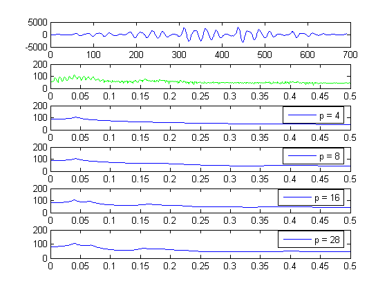
Linear predictive analysis of speech is demonstrated for various model orders. Notice how the model frequency response becomes more detailed and resembles the speech spectrum as the model order increases. The prediction error steadily decreases as the order of the model increases. There is an order however further from which any increases lead to minor decreases of the prediction error. The choice of the order basically depends on the sampling frequency and is essentially independent of the LPC method used. Usually, the model is chosen to have one pole for each kHz of the speech sampling frequency, due to vocal tract contribution and 3-4 poles to represent the source excitation spectrum and the radiation load. So for 16kHz speech a model order of 20 is usually suitable.

% Order values to test
orders = [4, 8, 16, 28];
l_ord = length(orders);

% Calculate the windowed speech spectrum
S = abs(fft(wx,1024));

subplot(l_ord + 2,1,1);
title('LP Analysis for various model orders')
plot(wx);
subplot(l_ord + 2,1,2);
plot(linspace(0,0.5,513), 20*log10(S(1:513)), 'g');

for o=orders
    [lpcoefs, e] = lpc(wx, o);
    % Estimated signal
    estx = filter([0 -lpcoefs(2:end)], 1, [wx; zeros(o,1)]);
    % Prediction error
    er = [wx; zeros(o,1)] - estx;
    erEn = sum(er.^2);

    % Frequency response of the model
    [H, W] = freqz(sqrt(erEn), lpcoefs(1:end), 513);

    subplot(l_ord + 2,1,find(orders==o) + 2);
    plot(linspace(0,0.5,513), 20*log10(abs(H)));
    legend(['p = ',int2str(o)]);
end

Published with MATLAB® 7.0